As in my previous blog, I have discussed white noise in time series data and I said that I will write some blogs on some of the few important concepts in time series forecasting and I would like to share some most important topics which are much needed for better forecasting and analysis. In this blog, I will discuss components of time series data, what is the decomposition of time series data, and how to achieve this in Python.
Basically, decomposition provides a very fine abstract knowledge(generalization) about time series data and it helps to understand the much clear problems during time series forecasting and analysis. Let’s first talk about time series components. There are two main components of abstraction for selecting forecasting methods which are systematic and non-systematic components. Systematic are those components of time series which have consistency in their patterns and can be described directly. Non-systematic are those components of time series that can not be described directly we have to do some pre-processing before describe/model them. A time-series includes three systematic components which include level, trend, and seasonality, and also include one non-systematic component which is noise in time series data.
Let’s just combine the time series components, though a series is a combination of level, trend, seasonality, and noise. For combining these components there are two models, one additive model and another is a multiplicative model. Trend and seasonality are optional because some time series does not have a trend and seasonality through time-series data must have level and noise in it. In the additive model the components are added together as below:
y(t) = Level + Trend + Seasonality + Noise
This model is linear where changes over time are consistently made by the same amount. A linear trend is a straight line. A linear seasonality has the same width and height of cycles. In multiplicative model components are combined together as bellow:
y(t) = Level × Trend × Seasonality × Noise
This model is nonlinear like exponential or quadratic and changes are not constant it can be increased or decrease over time. A nonlinear trend is a curved line and nonlinear seasonality has an increasing/decreasing frequency/amplitude over time.
Decomposition is mainly used for time series analysis, and as an analysis tool, it can be used to inform forecasting models on your problem. It provides a structured way of thinking about a time series forecasting problem, both generally in terms of modeling complexity and specifically in terms of how to best capture each of these components in a given model. Each of these components is something you may need to think about and address during data preparation, model selection, and model tuning. You may or may not be able to perfectly break down your specific time series as an additive or multiplicative model.
Real-world problems are messy and noisy. There may be additive and multiplicative components. There may be an increasing trend followed by a decreasing trend. There may be non-repeating cycles mixed in with the repeating seasonality components. Nevertheless, these abstract models provide a simple framework that you can use to analyze your data and explore ways to think about and forecast your problem.
There are different methods to automatically decompose a time series problem. The Statsmodels library provides an implementation of the decomposition method in a function called seasonal_decompose(). It requires that you specify whether the model is additive or multiplicative. After using the seasonal_decompose() function provided by statsmodels we can clearly view trend, seasonality, and residuals. In seasonal decompose() function there are different parameters the important parameter is model it indicates that if you want to decompose time series as an additive or multiplicative model as discussed above. Following is the basic use of seasonal_decompose() function.
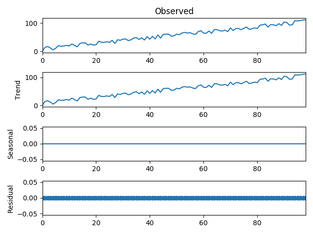
Let’s first take the linear additive model as shown below:
from statsmodels.tsa.seasonal import seasonal_decompose
series = [i+randrange(15) for i in range(1,100)]
decompose = seasonal_decompose(series, model= 'additive',period=1)
print(decompose.trend)
print(decompose.seasonal)
print(decompose.resid)
print(decompose.observed)
Following is the output produced by the above code snippet.
[ 14.  13.   6.  14.   6.   6.  12.  10.  20.  23.  24.  22.  22.  24.
  29.  24.  27.  26.  21.  22.  24.  33.  28.  36.  39.  34.  37.  36.
  40.  41.  38.  40.  42.  37.  37.  48.  47.  48.  41.  42.  42.  42.
  45.  48.  48.  59.  48.  57.  62.  54.  64.  58.  61.  59.  67.  60.
  68.  64.  63.  72.  65.  70.  74.  71.  74.  73.  77.  72.  69.  73.
  71.  72.  86.  75.  83.  84.  89.  81.  87.  82.  86.  89.  93.  87.
  97.  93.  92.  91.  98.  95. 100.  93.  96. 103. 101. 105. 104. 100.
 101.]
[0. 0. 0. 0. 0. 0. 0. 0. 0. 0. 0. 0. 0. 0. 0. 0. 0. 0. 0. 0. 0. 0. 0. 0.
 0. 0. 0. 0. 0. 0. 0. 0. 0. 0. 0. 0. 0. 0. 0. 0. 0. 0. 0. 0. 0. 0. 0. 0.
 0. 0. 0. 0. 0. 0. 0. 0. 0. 0. 0. 0. 0. 0. 0. 0. 0. 0. 0. 0. 0. 0. 0. 0.
 0. 0. 0. 0. 0. 0. 0. 0. 0. 0. 0. 0. 0. 0. 0. 0. 0. 0. 0. 0. 0. 0. 0. 0.
 0. 0. 0.]
[ 14.  13.   6.  14.   6.   6.  12.  10.  20.  23.  24.  22.  22.  24.
  29.  24.  27.  26.  21.  22.  24.  33.  28.  36.  39.  34.  37.  36.
  40.  41.  38.  40.  42.  37.  37.  48.  47.  48.  41.  42.  42.  42.
  45.  48.  48.  59.  48.  57.  62.  54.  64.  58.  61.  59.  67.  60.
  68.  64.  63.  72.  65.  70.  74.  71.  74.  73.  77.  72.  69.  73.
  71.  72.  86.  75.  83.  84.  89.  81.  87.  82.  86.  89.  93.  87.
  97.  93.  92.  91.  98.  95. 100.  93.  96. 103. 101. 105. 104. 100.
 101.]
From the above output, you can clearly see that there is no seasonality and residuals. As we use the additive model that’s why there is a linear graph as shown below.
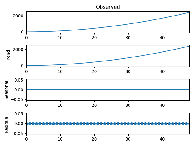
Now let’s take the multiplicative model which will produce non-linear results as shown below:
series = [i**2.0 for i in range(1,50)]
decompose = seasonal_decompose(series,model='multiplicative',period=1)
print(decompose.trend)
print(decompose.seasonal)
print(decompose.resid)
print(decompose.observed)
Following is the output from the above code snippet:
[1.000e+00 4.000e+00 9.000e+00 1.600e+01 2.500e+01 3.600e+01 4.900e+01
6.400e+01 8.100e+01 1.000e+02 1.210e+02 1.440e+02 1.690e+02 1.960e+02
2.250e+02 2.560e+02 2.890e+02 3.240e+02 3.610e+02 4.000e+02 4.410e+02
4.840e+02 5.290e+02 5.760e+02 6.250e+02 6.760e+02 7.290e+02 7.840e+02
8.410e+02 9.000e+02 9.610e+02 1.024e+03 1.089e+03 1.156e+03 1.225e+03
1.296e+03 1.369e+03 1.444e+03 1.521e+03 1.600e+03 1.681e+03 1.764e+03
1.849e+03 1.936e+03 2.025e+03 2.116e+03 2.209e+03 2.304e+03 2.401e+03]
[0. 0. 0. 0. 0. 0. 0. 0. 0. 0. 0. 0. 0. 0. 0. 0. 0. 0. 0. 0. 0. 0. 0. 0.
0. 0. 0. 0. 0. 0. 0. 0. 0. 0. 0. 0. 0. 0. 0. 0. 0. 0. 0. 0. 0. 0. 0. 0.0.]
[0. 0. 0. 0. 0. 0. 0. 0. 0. 0. 0. 0. 0. 0. 0. 0. 0. 0. 0. 0. 0. 0. 0. 0.
0. 0. 0. 0. 0. 0. 0. 0. 0. 0. 0. 0. 0. 0. 0. 0. 0. 0. 0. 0. 0. 0. 0. 0.0.]
[1.000e+00 4.000e+00 9.000e+00 1.600e+01 2.500e+01 3.600e+01 4.900e+01
6.400e+01 8.100e+01 1.000e+02 1.210e+02 1.440e+02 1.690e+02 1.960e+02
2.250e+02 2.560e+02 2.890e+02 3.240e+02 3.610e+02 4.000e+02 4.410e+02
4.840e+02 5.290e+02 5.760e+02 6.250e+02 6.760e+02 7.290e+02 7.840e+02
8.410e+02 9.000e+02 9.610e+02 1.024e+03 1.089e+03 1.156e+03 1.225e+03
1.296e+03 1.369e+03 1.444e+03 1.521e+03 1.600e+03 1.681e+03 1.764e+03
1.849e+03 1.936e+03 2.025e+03 2.116e+03 2.209e+03 2.304e+03 2.401e+03]
As we use a multiplicative model that’s why there is a nonlinear graph which is quadratic as shown below:
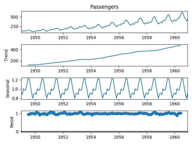
Let’s take a real-world Airline Passengers dataset and analysis that. This dataset describes the total number of airline passengers over time.
import pandas as pd
import matplotlib.pyplot as plt
from statsmodels.tsa.seasonal import seasonal_decompose
series = pd.read_csv('airline-passengers.csv',header=0,index_col=0,parse_dates=True,squeeze=True)
decomposed = seasonal_decompose(series,model='multiplicative')
print(series.head(10))
decomposed.plot()
plt.show()
Following is the top 10 data points output of above code snippet:
Month
1949-01-01 112
1949-02-01 118
1949-03-01 132
1949-04-01 129
1949-05-01 121
1949-06-01 135
1949-07-01 148
1949-08-01 148
1949-09-01 136
1949-10-01 119
Name: Passengers, dtype: int64
Following is the graphical representation of the above mentioned airline-passengers data.
That’s it for today I hope you have learned about components of time series, what is decomposition and how to achieve automatically decomposition of our time series in Python.
